White Paper

Recommendations for Overcoming the Limitations of Capacity Tests of Utility-Scale Photovoltaics Projects

The gathering of sufficient valid data points to meet photovoltaic project capacity test procedures can present major challenges. Mitigation strategies are available to overcome these challenges. These include using wider irradiances ranges, higher resolution data, and stowing tracked arrays.


When photovoltaic project capacity test methodologies most widely used in the U.S. are combined with current design approaches (trackers, high DC:AC ratios, bifacial modules) and are more commonly located outside the desert Southwest, inherent challenges arise in obtaining sufficient data points to meet typical capacity test procedure requirements.

These challenges include inverter and/or plant clipping during most of the day, low irradiance in the winter, external shading outside of clipping hours, shading during backtracking, and rapidly changing irradiance during backtracking.

Irradiance filtering is used to minimize data points with nonlinearities and/or instabilities. These nonlinearities are summarized with a view to understanding the impact of using data points outside the normally accepted criteria.


Read The White Paper

When photovoltaic project capacity test methodologies most widely used in the U.S. are combined with current design approaches (trackers, high DC:AC ratios, bifacial modules) and are more commonly located outside the desert Southwest, inherent challenges arise in obtaining sufficient data points to meet typical capacity test procedure requirements.

These challenges include inverter and/or plant clipping during most of the day, low irradiance in the winter, external shading outside of clipping hours, shading during backtracking, and rapidly changing irradiance during backtracking.

Irradiance filtering is used to minimize data points with nonlinearities and/or instabilities. These nonlinearities are summarized with a view to understanding the impact of using data points outside the normally accepted criteria.

Several mitigation strategies are presented to address these challenges. Some involve modifications to the procedures — including larger irradiance ranges, higher resolution data and fewer data points required — and some involve temporary modifications to the operations of a PV plant such as stowing trackers flat, or reducing DC capacity. Within the appropriate limitations, these mitigation strategies can be used with minimal impact in the results of the test or with only slightly higher uncertainty.

Photovoltaic Project Capacity Tests

A capacity test is a key acceptance test for most large photovoltaic (PV) projects and is often a condition of substantial completion. The timely and successful completion of the capacity test is thus of great interest to the contractor as well as to the system owner and third parties such as regulators, utilities and finance partners. The capacity test methodologies most commonly used require a regression analysis with reasonably stable and linear data. However, weather conditions and PV system designs are often such that it is difficult or impossible to obtain enough valid data points in the time period often required by the schedule. There are various strategies that strive to address and mitigate the challenges in obtaining enough valid data points, while still providing a high level of accuracy in the results.

A capacity test is designed to measure the DC capacity of the PV array as adjusted by the DC and AC losses and compare the result with the design capacity and losses. Capacity tests measure environmental conditions and project output power, and typically create a regression of power versus plane of array (POA) irradiance, modified implicitly or explicitly by module temperature, depending on the test protocol. The data are strongly filtered to support a linear regression and avoid outliers. The same filters are applied to both the measured and modeled data and the regression equations from each data set are solved for the same reporting conditions (RCs) and compared.

The leading industry standard test for capacity testing in the U.S. is ASTM E2848, “Standard Test Method for Reporting Photovoltaic Non-Concentrator System Performance.” A key component of ASTM E2848 is the principle that the target capacity should be based on the energy production model results at the same reporting conditions, rather than either the DC or the AC wattage at Standard Test Conditions (STC) as was the industry practice in the early 2010s. In addition, the filters to maintain a linear dataset are described in moderate detail.

The International Electrotechnical Commission (IEC) in IEC TS 61724-2 provides guidelines for alternate capacity tests and uses the term “target reference conditions” (TRCs) rather than “reporting conditions.” IEC 61724 also recognizes the problem of evaluating test data at STC, which would often be a “constrained” rather than an “unconstrained” condition with a TRC at a lower irradiance. This test specification also covers data filtering similar to that presented by the ASTM standard.

Both approaches are based on the principle that power output is very closely proportional to plane of array (POA) irradiance and secondarily impacted by PV cell temperature — with decreasing power as the temperature rises and vice versa as it falls.

The ASTM approach uses a multivariate regression using the following environmental inputs:

  • POA irradiance
  • Ambient temperature
  • Wind speed

The logic behind these inputs is that the POA irradiance is the main driver and all three variables contribute to cell temperature.

The IEC approach also depends on POA irradiance and cell temperature — derived either from module temperature measurements or theoretical calculations based on the same environmental inputs as above. The observations already outlined apply to both the ASTM approach and the IEC unconstrained approach.

Nonlinear Aspects of PV Systems

There are numerous nonlinear phenomena that can impact the accuracy of a capacity test. The main ones include the following:

Inverter Clipping and/or Point of Interconnection (POI) Limitations

When either the inverter power output limit or the POI limit is reached, increasing POA irradiance (or dropping the cell temperature) will produce no increase in power. This results in a graph similar to Figure 1.


Figure 1: Temperature-Adjusted Power.

To avoid these nonlinearities, all data points at or above these output limits are excluded from the dataset. With the drive to maximize the utilization of the AC capacity of a plant, this means that under good solar conditions on a tracking system almost all data points during the day are excluded. This is often the main factor limiting the collection of valid data points and can be exacerbated by the use of bifacial modules unless the nameplate DC capacity is reduced accordingly.

PV Module and Inverter Efficiency Curves

The efficiency curve of most PV modules is reasonably linear from approximately 400-1000 W/m2 but drops off significantly below that range, especially as it approaches zero irradiance. See examples in Figures 2 and 3.

Figure 2: Relative Efficiency With Respect to STC.

Figure 3: Absolute Efficiency With Respect to Irradiance.

Inverter Efficiency With Respect to Irradiance

Similar to PV modules, the typical efficiency curve of inverters is reasonably linear from about 20% to 80% of its rated output. It drops off slightly as it reaches 100% and strongly as it approaches zero (see Figure 4). This drop-off near 100% of capacity can be exacerbated by increasing cooling fan power consumption at high power outputs.

Figure 4: Inverter Efficiency vs. Power Output.

These nonlinearities can be mitigated by using only irradiances above a certain minimum value typically in the 200–400 W/m2 range. However, this may become a major issue when testing PV plants in the winter, especially the further from the equator that a plant is located. In addition, the elimination of points near the rated power are often separately eliminated to avoid any points involving clipping.

Incident Angle Effects

As sunlight hits a PV module at a more oblique angle, more light is reflected off the module and less is absorbed by the solar cells (see Figure 5). Pyranometers experience a similar effect.

This nonlinearity is largely avoided by using only times with high irradiance where the incident angle is usually more direct (normal), though this is rarely explicitly filtered.

Figure 5: Incidence Angle Modifier.

I2R losses

Power losses through cables are proportional to the square of the current and the resistance (R) of the cables. There is a similar effect with the load losses in transformers. Fortunately, those combined losses are typically on the order of 4% to 5% of a plant’s output so the impact of this nonlinearity is low. However, this impact can be mitigated by using data from a limited portion of the total power range. ASTM recommends 40% but allows a larger portion if needed to collect enough valid data points.

Instrumentation

Most measuring instruments are not perfectly linear, especially near their zero readings. This is not usually a material factor except at low irradiance and power levels.

Data Scatter

Data scatter can be caused by a number of factors, including:

  • Rapidly changing irradiance, which will produce an immediate response in the output power but a much slower response in the cell temperatures.
  • Different wind directions, which may cool the PV modules more or less effectively.
  • Different or changing sky temperatures, which will also impact the temperature of the PV modules.
  • Variable auxiliary loads (e.g., tracker motors), which can cause “noise” in the power output data.
  • Tracker angle variability.
  • Variable shading of a site.

Scenarios Limiting the Collection of Valid Data Points Inverter/POI Limiting

The most obvious nonlinearity in a PV system is inverter clipping and/or POI limitations, particularly during good solar conditions when trackers are used. Such systems have an M-shaped irradiance curve and can hit the power output limit within 1 hour to 1.5 hours of sunrise with a similar ramp-down before sunset (see the Tracking vs Stowed graph, Figure 6). When low irradiance filters are applied, this may leave only small portions of the ramp-up and ramp-down time periods available for use in the capacity test. These time periods are essentially during backtracking and thus the incident angle effects can be a greater factor than normal.

PV systems are frequently “overbuilt” with high DC:AC ratios (> 1.3–1.4, depending on climate), which cause the systems to reach the power output limits at relatively low irradiances (e.g., 850 W/m2 rather than 950 W/m2 as was more typical in the early years of utility-scale solar when PV modules were much more costly). Bifacial modules can also cause the system to reach its power output limit at a lower irradiance, especially if the albedo is high, such as with snow. A variant of this issue is having widely varying DC:AC ratios on different inverters in the same project. The inverter with the highest DC:AC ratio will clip first and cause any such data points to be eliminated.

Environmental Conditions

Low irradiance can be an inherent factor when performing a capacity test in the winter where the POA irradiance may peak between 950 W/m2 on a sunny day and even lower during overcast conditions. Low peak irradiance limitations can often not be avoided — especially considering tax year deadlines — but overcast days can be avoided though with resulting schedule delays. These scheduling delays may even require that a full capacity test be made a final completion requirement rather than more typically as a substantial completion requirement.

Topography and shading can be issues, especially as more and more PV plants are being built in forested areas, often with undulating terrain. Time periods with shading are usually removed from the analysis. In some cases with trackers, there may be situations when no or almost no time periods will have valid data points — some removed for shading and the rest for clipping.

Irradiance instability by variable cloudiness — especially with fast-moving clouds — will generally be filtered out by the stability criteria. This instability can be either temporal or spatial or both. The filtering criteria are typically based on differences amongst the irradiance sensors at the same time (spatial) or changes in the irradiance over time (temporal) or both.

Data Sampling

A capacity test’s prescription of the time stamps to be used can also eliminate data points. The typical resolutions used are 1, 5, and 15 minutes. Clearly if the only possible time periods for valid data points are during the ramp-up and ramp-down times, the 15-minute data points will prove to have temporally unstable irradiance and will be eliminated. Irradiance can change as much as 10-15 W/m2 per minute in extreme cases. In those cases, even 5-minute data may prove “unstable” or require modification of the defined variability thresholds.

Proposed Mitigation Strategies

Placing trackers in a fixed, horizontal position is probably the most straightforward mitigation strategy and has been widely used. By placing the trackers into a horizontal stow position, it temporarily turns the array into a fixed array with a sinusoidal power output curve rather than an M-shaped curve, with the power curve flattened to a trapezoid. In Figure 6, the difference in this day is 86 points between 400 and 800 W/m2 tracking and 227 points stowed. This project begins clipping at about 800 W/m2. With these higher DC:AC ratio arrays, typically more than an additional hour of valid irradiance may be captured on either end of the day by placing the trackers in stow. The changes in irradiance per minute are also lower, on the order of 3-4 W/m2 per minute. One can thereby avoid these points being filtered out by the power limitation filter and, on sunny days, by the irradiance temporal filter.

Based on field experience, performance testing with the trackers stowed is worth considering when the model indicates the project will be power limited at about 850 W/m2. If the project will be power limited at 800 W/m2 or below, stowing during performance testing is recommended.

Figure 6: Tracking vs. Stowed.

The main disadvantage is the loss of energy production during the test days. This will typically be in the 10% to 40% range depending on the time of year, location, and design. A second disadvantage is an increased incident angle effect, especially during the winter or far from the equator. This strategy is usually needed during spring, summer and fall.

A procedural disadvantage is that the energy model (e.g., PVsyst) needs to have a special variant run with the trackers in the horizontal position. However, if the PVsyst model is already set up, this is quite easy to do.

Use 1-Minute Resolution Data

The use of 1-minute data points can make ramp-up and ramp-down time periods and temporally unstable cloudy time periods usable for analysis. The main disadvantage to this approach is the thermal time lag with module temperatures. For example, if the module temperatures are lagging the irradiance by 2°C and the modules have a maximum power coefficient of -0.4%/°C, the impact will reflect an error of 0.8% higher actual power when irradiance is increasing and 0.8% lower actual power when irradiance is decreasing. In most cases, the number of data points will be approximately the same in both directions, thus canceling out the errors. Ideally the resulting regression curve will have two parallel lines with the correct regression on a line halfway between them and will so be calculated (Figure 7). In reality, a “thick” plot of data points can usually be seen commingling the morning and afternoon points. As such, the resulting solution of the regression equation will still be valid provided the data set includes relatively equal amounts of increasing and decreasing irradiance periods.

Figure 7: Power Adjusted to 45°C Cell Temperature.

Increasing the Range of Irradiance Values

Lowering the minimum irradiance used can be very useful in the winter and farther from the equator when irradiances above 400 W/m2 are rare or even impossible, even on a sunny day. A common value used is 300 W/m2. The main disadvantage to this approach is that PV module efficiency becomes noticeably nonlinear at that range though not as nonlinear as in the 100-300 W/m2 range. However, with the ASTM E2848 regression, the impact of nonlinearities is reduced by 1) evaluating the regression at an irradiance within the measured data, and 2) using a limited range of irradiances where the effect of the nonlinearities is also limited. However, the use of low irradiances with regressions evaluated at 1,000 W/m2 or other high irradiance values is not recommended due to the higher impact of the nonlinearities including extrapolation error.

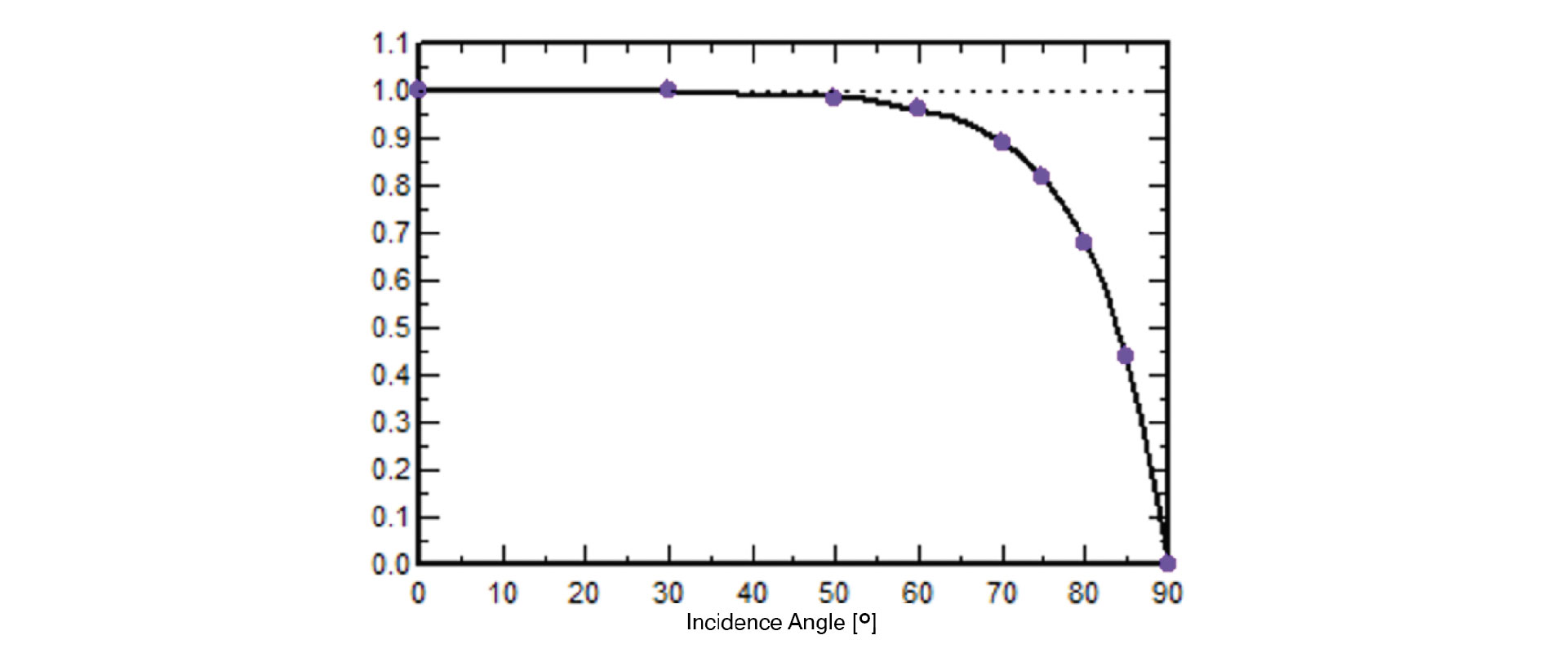
A second disadvantage is that the incident angle modifier (IAM) losses are greater (and nonlinear) with low sun angle, introducing additional errors. However, low irradiance due to overcast conditions does not have this disadvantage and can be used. Sunny time periods with high IAM losses can be filtered out based on time stamps.

Increasing the range of irradiance values at levels higher than 400 W/m2 used in the test is actually recognized in ASTM E2848. That standard recommends using irradiances only ±20% from the RC irradiance but supports the use of expanding the range in order to collect more data points.

Temporarily Reducing the DC Capacity

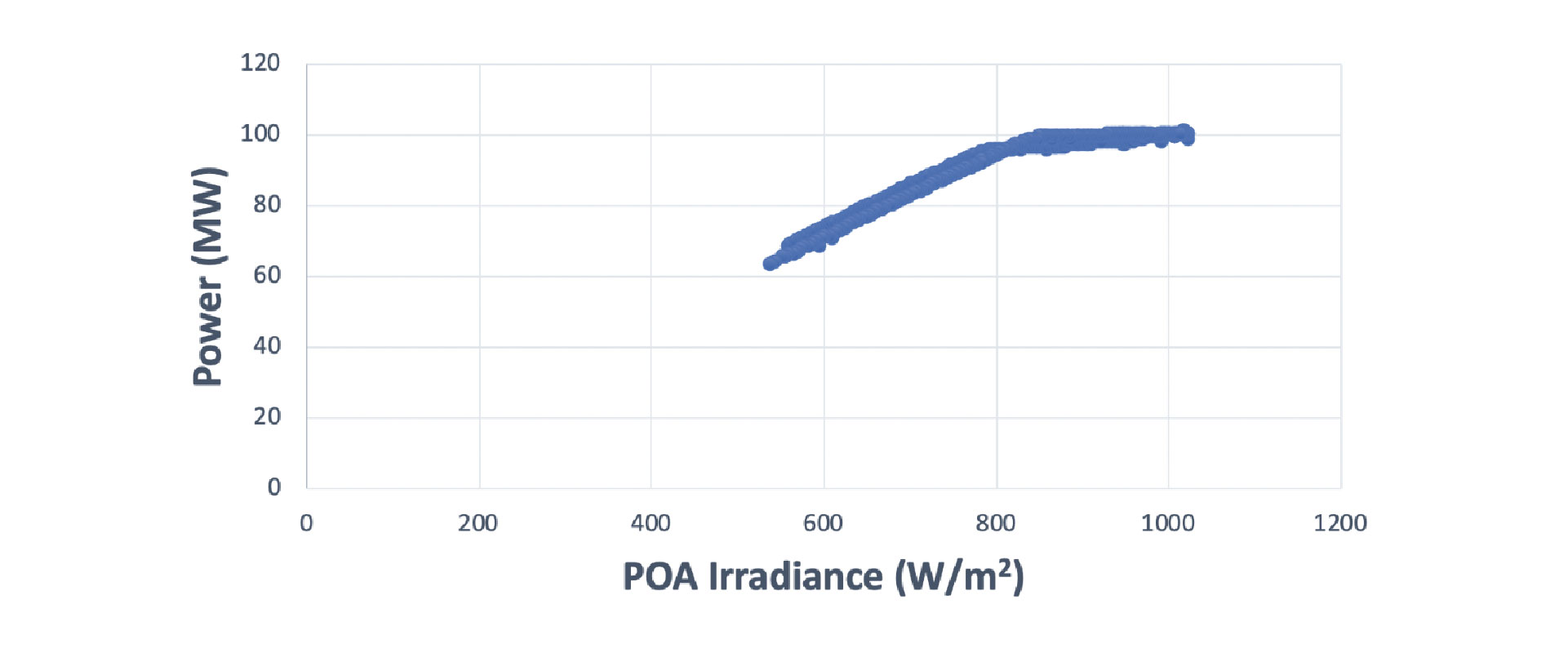
When clipping is an issue, rather than stowing the trackers, the DC capacity of the PV arrays can be temporarily reduced by opening the switches on a limited number of combiner boxes. The PVsyst model would also need to be modified to reflect the reduced DC capacity. In this case, the overall results would need to be scaled in order to truly reflect the plant’s full capacity. Ideally, the offline combiner boxes would be rotated with online combiner boxes and the test run twice. This would allow a test of every portion of the PV arrays with results combined to present the full capacity. Less ideally, the current output of the temporarily offline combiner boxes could be compared with the online ones under similar conditions to ascertain that the power outputs are indeed proportional.

Use of Limited Data Points With Horizon or Near Shading

While not ideal, the limited use of data from time periods with minimal shading from trees or other objects can be used, especially if the plant goes rapidly from shaded periods to clipping. The shading percentage can be calculated by PVsyst and/or observed in the field. The authors’ experience with this approach is that allowing time stamps with shading less than 3% can still produce usefully accurate regression results. If based on PVsyst hourly data, it is prudent to use measured data only from the second half-hour of the corresponding time stamps in the morning and the first half-hour in the afternoon to avoid time periods with shading more than 3%. If this approach is used, the test uncertainty will increase and should be acknowledged.

Preferably, one of the other mitigation strategies such as stowing the tracker or reducing the DC capacity should be tried first to avoid the additional errors and uncertainties in using data with limited shading.

Reducing the Number of Data Points Used in the Regression

When the data are relatively consistent, a reduced number of data points can be used and still provide a valid regression. This is already done with PVsyst data since they are usually in an hourly format. Similarly, as few as 50 measured 1-minute or 5-minute data points can produce good regressions with consistent data. The linearity of the data can be evaluated via the coefficient of determination (R2 where R is the Pearson correlation coefficient). While other data consistency parameters can be used as a supplement, an R2 of 0.93 or above can be considered a reasonable lower limit. When this approach is used, a good additional validation practice is to identify two or more actual data points close to the RCs and compare their output power to the regression results. Collecting data from at least two or three days, as specified in the IEC and ASTM standards, respectively, is an important requirement for this test modification. All of these factors must be considered when agreeing to a reduced number of data points, and it is not possible to predetermine an absolute minimum a priori.

Conclusion

The capacity test methodologies most widely used in the U.S. combined with current design approaches (trackers, high DC:AC ratios, bifacial modules) and the increase in PV project locations outside the desert Southwest present inherent challenges in obtaining sufficient data points to meet the capacity test procedure requirements.

There are several mitigation strategies that can be used to address this challenge. Some involve modifications to the procedures such as larger irradiance ranges, higher resolution data or fewer points required. Some involved temporary modifications to the operations of the PV plant such as stowing trackers flat or reducing DC capacity. Within the appropriate limitations, these mitigation strategies can be used with minimal impact in the results of the test or with only slightly higher uncertainty.

Video Column Complete


Cool Video Headline Goes Here

video description goes here. video description goes here


Authors

Grant Reasor

Senior Electrical Engineer

Jessica Forbess

Principal Engineer, Sunshine Analytics